Week 2: September 16, 2024
This blog is an ongoing project for Professor Ryan Enos' Election Analytics Course at Harvard College (GOV 1347, Fall 2024). It will be updated weekly with posts analyzing how different features impact the likelihood of Kamala Harris (D) or Donald Trump (R) winning the 2024 U.S. Presidential Election or winning specific states in the election. The blog will culminate in a final predictive model for the outcome of the general election.Context & Question
In his successful 1992 campaign for the U.S. Presidency, Bill Clinton is quoted as saying "it's the economy, stupid." Clinton implied that, in a strong economy, voters would favor an incumbent candidate/party, and vice versa in a weak economy. There are several philosophies about what constitutes a "strong economy." Changes in GDP, in GDP per capita, unemployment rate, and inflation rate are all indicators. In this post, I'm interested in looking at the strength of the U.S. Dollar (USD) relative to the currencies of major trading partners and allies, and seeing if it holds predictive power in presidential elections.The Data
The Federal Reserve Bank of St. Louis publishes the daily exchange rates between the U.S. dollar and a variety of other currencies. I chose to use data about the Japanese Yen, the Chinese Yuan Renminbi, the British Pound, and the Euro. The span of data available for each currency is summarized below:| Currency | Start of Data |
|---|---|
| Japanese Yen | January 4, 1971 |
| British Pound | January 4, 1971 |
| Chinese Yuan | January 2, 1981 |
| Euro | January 4, 1999 |
The American Economy is linked to the Japanese Yen through carry-trading. The Yen has historically had no interest rate, making it an attractive currency for investors to buy, place in stocks or bonds, and then exchange for USD (or another foreign currency) before collecting the returns on their investments. However, changes in the value of the Yen can send the U.S. stock market into turmoil, as happened in the first week of August, 2024. Another reason to use the Yen is the mutual defense agreement between the U.S. and Japan. Though remnant of the post-World War II era, part of this agreement’s appeal is that the U.S. earns a profit selling defense technology to Japan. In doing so, it bolsters the nation’s capacity to defend itself and reduces the chance that the U.S. will have to intervene. In this sense fluctuations in the Yen can be foreboding about the U.S. economy. A weak Yen may cost the U.S. in defense exports, and simultaneously make U.S. intervention in Japan seem more likely, especially in the face of rising tensions between China and Taiwan, and the North Korean threat in southeast Asia.
I chose to use the Chinese Yuan because China accounts for the greatest portion of U.S. imports. An especially strong Yuan might lead to high prices for everyday goods in the U.S., causing the entire economy to struggle. Further, since China does not operate under a free market economy, the value of the Yuan can be telling about the strength of the state/its military. U.S. relations with China have become a partisan issue in the time for which we have data. 1971 was a landmark year as President Nixon lifted travel restrictions for Americans hoping to visit China. In the time since, relations have been strained by the Tianenman Square massacre, the 1996 crisis in the Taiwan Strait, and several 21st-century naval face offs. Both Democratic and Republican presidents have had to deal with these issues, and have their own ways of responding. President Biden, for example, has said publicly that he would send U.S. Troops to defend Taiwan should it become necessary. Former President Trump has proposed major tariff increases on Chinese imports in an effort to slow its economy and its growth into a global power. Here we focus on what the value of the Yuan implies about the U.S. economy, keeping the idea that a strong Yuan is harmful to everyday prices and a weak Yuan is beneficial for the U.S. economy, assuming trade is not curbed by international conflict.
I chose to use the Euro and the British Pound because of the alliances that the U.S. maintains with the United Kingdom (UK) and nations in the European Monetary Union (EMU). The values of their currencies can be telling about whether the U.S. economy is at risk because of one of its unique dependencies or commitments overseas. They also indicate how accessible travel/tourism to the popular destinations that use these currencies is to Americans, which generally improves quality of life and makes voters more optimistic.
Exploratory Analyses
Visualizing Four Currencies Against the Dollar Over Time
# load libraries
library(dplyr)
##
## Attaching package: 'dplyr'
## The following objects are masked from 'package:stats':
##
##     filter, lag
## The following objects are masked from 'package:base':
##
##     intersect, setdiff, setequal, union
library(ggplot2)

# load the data
dollar_to_yen <- read.csv("DEXJPUS.csv")
dollar_to_yuan <- read.csv("DEXCHUS.csv")
dollar_to_lb <- read.csv("DEXUSUK.csv")
dollar_to_euro <- read.csv("DEXUSEU.csv")
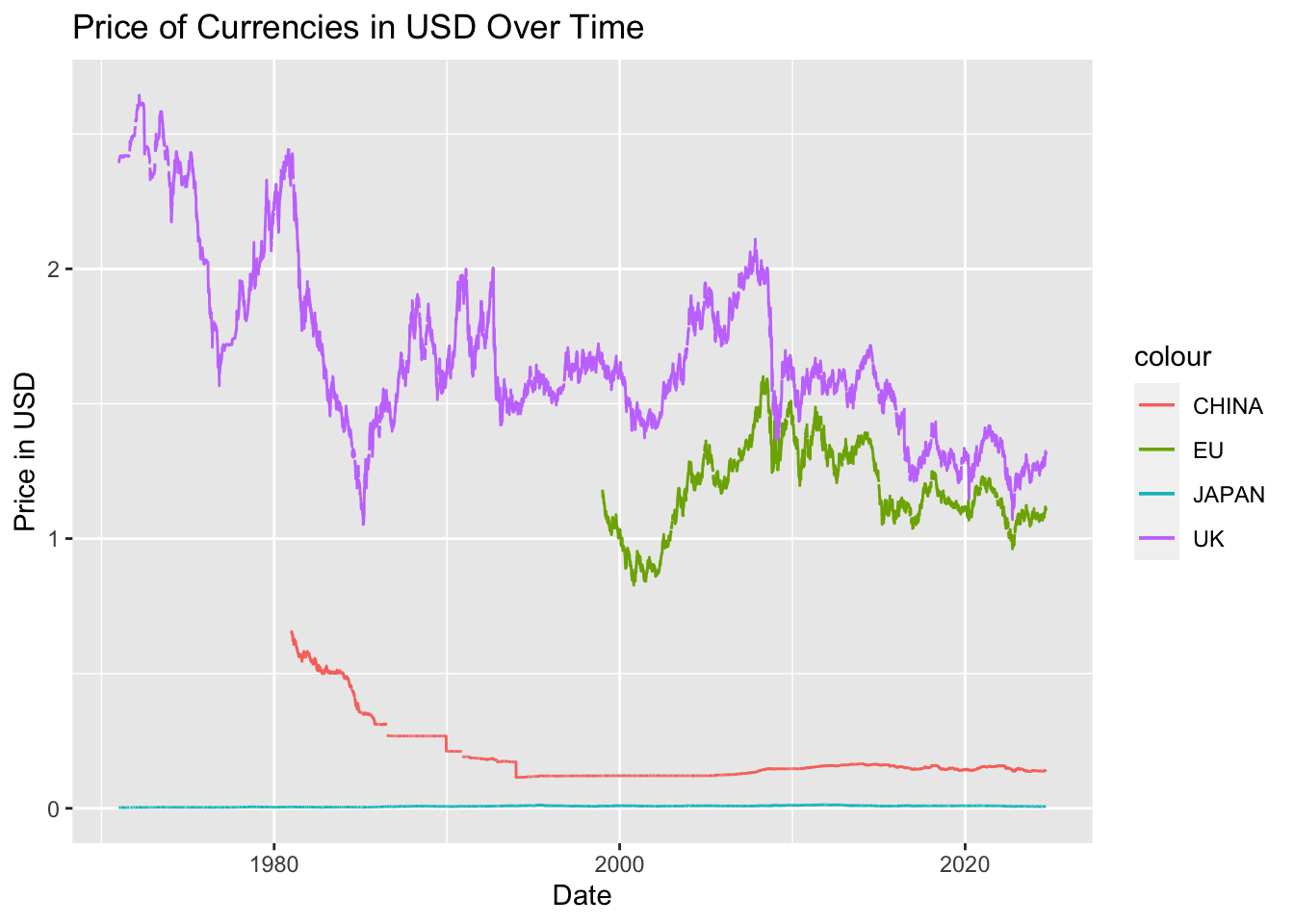
As provided, the data for China and Japan reflects the price of a Dollar in Yen and Yuan, respectively. The data for the EMU and UK reflects the price of a Euro or a Pound, respectively, in USD. To make these consistent, I inverted the metric for the Yuan and Yen. This way, all datasets have a column reflecting the price of a foreign currency in USD. A value less than one indicates that the Dollar is stronger than the other currency; a value above one indicates that the Dollar is weaker.
# coerce all exchange rates to numeric
dollar_to_yen$DEXJPUS <- as.numeric(dollar_to_yen$DEXJPUS)
dollar_to_yuan$DEXCHUS <- as.numeric(dollar_to_yuan$DEXCHUS)
dollar_to_lb$DEXUSUK <- as.numeric(dollar_to_lb$DEXUSUK)
dollar_to_euro$DEXUSEU <- as.numeric(dollar_to_euro$DEXUSEU)

# invert Japan and China Exchange Rates
dollar_to_yen$DEXUSJP <- 1 / dollar_to_yen$DEXJPUS
dollar_to_yuan$DEXUSCH <- 1 / dollar_to_yuan$DEXCHUS
# visualize the price of each currency in dollars over time
# aggregate data
all_currencies <- full_join(dollar_to_yen, dollar_to_lb, by = "DATE") %>%
                  left_join(dollar_to_yuan, by="DATE") %>%
                  left_join(dollar_to_euro, by="DATE") %>%
                  select(!c(DEXCHUS, DEXJPUS)) %>%
                  # convert to datetime
                  mutate(DATE = as.Date(DATE))

ggplot(data=all_currencies)+
  geom_line(mapping=aes(x=DATE, y=DEXUSJP, color = "JAPAN")) +
  geom_line(mapping=aes(x=DATE, y=DEXUSCH, color = "CHINA")) +
  geom_line(mapping=aes(x=DATE, y=DEXUSEU, color = "EU")) +
  geom_line(mapping=aes(x=DATE, y=DEXUSUK, color = "UK")) +
  ylab("Price in USD") +
  xlab("Date") +
  ggtitle("Price of Currencies in USD Over Time")
The following dataset contains the Democratic and Republican shares of the popular vote and electoral college–as well as the name of the incumbent party–for every election since 1952. It is trimmed to only include elections for which we have Fed data about the value of the USD (i.e., elections since 1972).
# load election data
election_outcomes <- read.csv("ElectionResults2.csv") %>%
                     filter(Year > 1971)
The data about USD value over time are roughly continuous between the earliest record and the latest record in 2024. Data about the presidential election outcomes since 1972 are discrete since U.S. presidential elections are held every four years. In order to use the value of the Dollar as a predictor of election outcomes, I will define a few aggregate metrics from the data. For each election, the strength of the USD will be captured in a single value and I’ll be able to analyze whether that metric is a reasonable predictor of election outcome.
Aggregate Metric: Average Value of the USD
Below I define the average value of the U.S. Dollar relative to each of the other four currencies, respectively. I calculate this twice: I calculate the average value of the USD over a four-year period (i.e., the incumbent's entire term), then I calculate the average value over the year leading up to the election. This reflects the finding from Achen and Bartels (2017) that voters tend to prioritize the short-term state of the economy, if they consider economic factors at all when casting a ballot.# import extra library for formatting
library(stringr)
# find the average value of USD in the 4 years leading up to each election
all_currencies$YEAR <- strftime(all_currencies$DATE, format="%Y")
exchange_rates <- c("DEXUSJP", "DEXUSCH", "DEXUSUK", "DEXUSEU")
new_variables4y <- c("USD4YJP", "USD4YCH", "USD4YUK", "USD4YEU")
new_variables1y <- c("USD1YJP", "USD1YCH", "USD1YUK", "USD1YEU")
# set up variables for USD value relative to all currencies
for (i in seq(1,4)) {
len <- length(election_outcomes$Year)
election_outcomes[[new_variables4y[i]]] <- rep(NA, len)
election_outcomes[[new_variables1y[i]]] <- rep(NA, len)
}
# 4-Year Metric
for (i in seq(1,length(election_outcomes$Year))) {
year <- election_outcomes$Year[i]
# start of Year (year - 4)
lowest_date <- year - 4
# November 1 of election year
highest_date <- as.Date(str_glue("11/01/",year), "%m/%d/%Y")
for (j in seq(1,4)) {
election_outcomes[[new_variables4y[j]]][i] <- mean(all_currencies[[exchange_rates[j]]][(all_currencies$DATE <= highest_date) & (strftime(all_currencies$DATE, format="%Y") >= lowest_date)], na.rm=TRUE)
}
}
# 1-Year Metric
for (i in seq(1,length(election_outcomes$Year))) {
year <- election_outcomes$Year[i]
# November 1 of election year
highest_date <- as.Date(str_glue("11/01/",year), "%m/%d/%Y")
for (j in seq(1,4)) {
election_outcomes[[new_variables1y[j]]][i] <- mean(all_currencies[[exchange_rates[j]]][(all_currencies$DATE <= highest_date) & (strftime(all_currencies$DATE, format="%Y") >= year)], na.rm=TRUE)
}
}
Analysis & Results
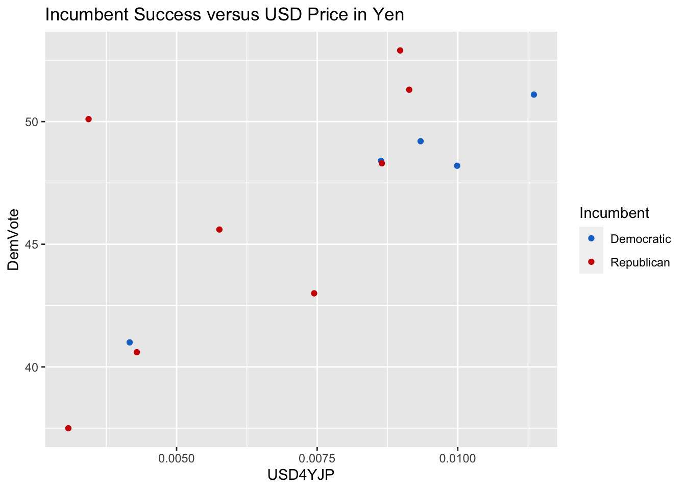
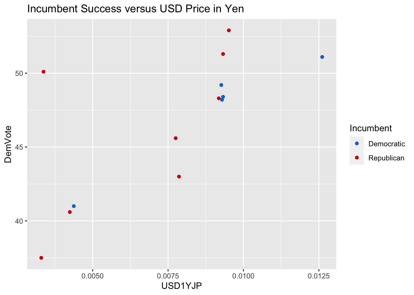
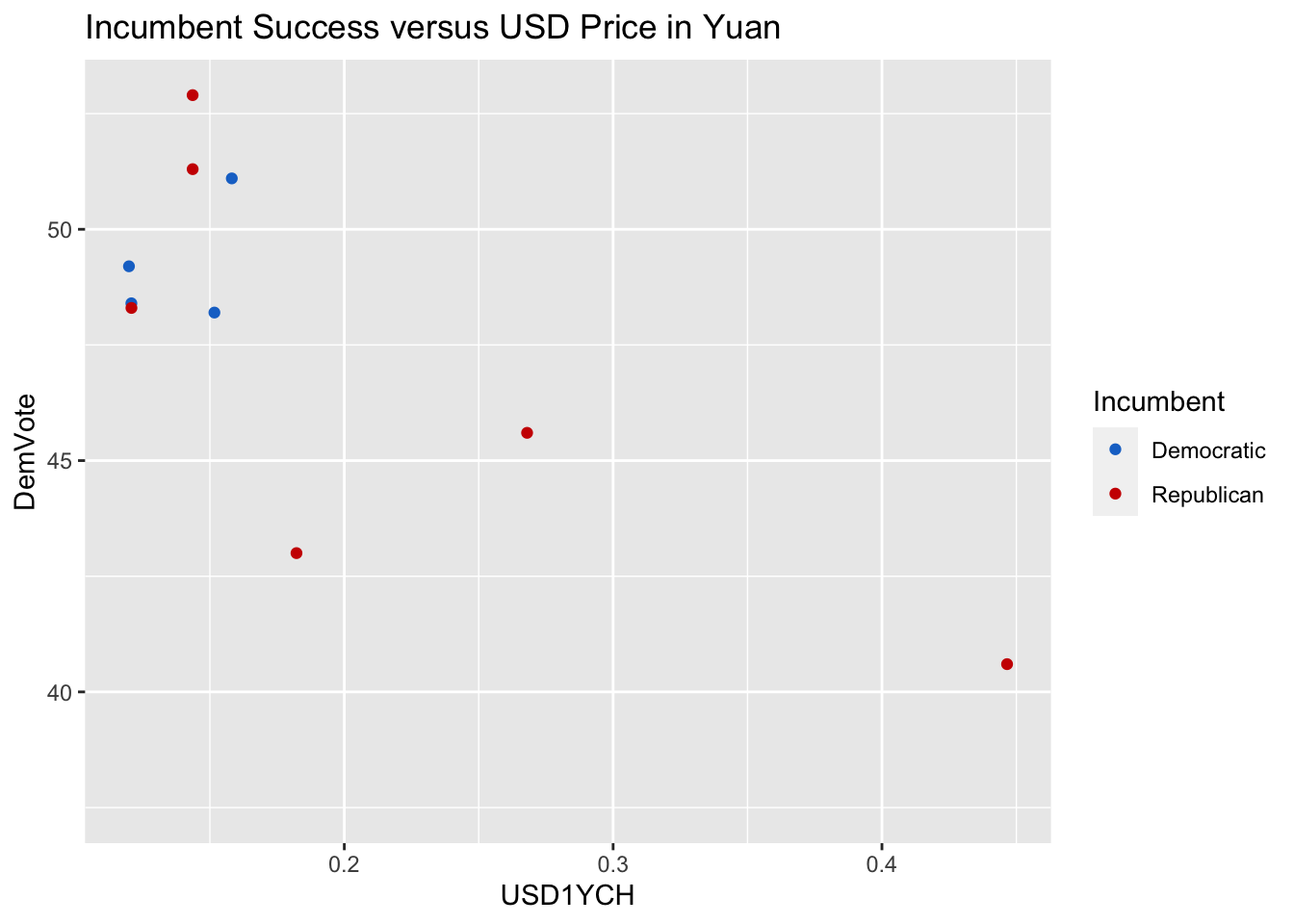
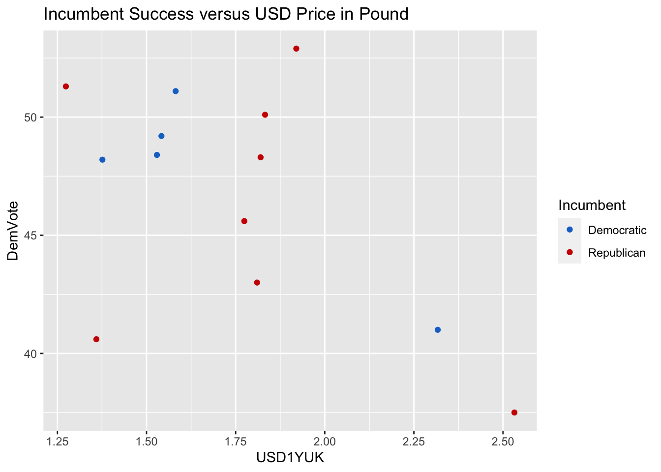
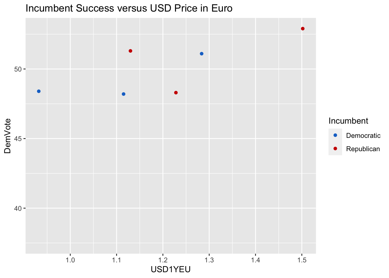
The plots below show the Democratic share of the popular vote (Y-axis) relative to the 4-year average value in the USD of each of the four currencies examined (X-axis).yen_plot <- ggplot(data=election_outcomes) + geom_point(aes(x=USD4YJP, y=DemVote, color=Incumbent, label=Year)) + scale_color_manual(breaks = c("Democratic", "Republican"), values = c("dodgerblue3", "red3")) + ggtitle("Incumbent Success versus USD Price in Yen")
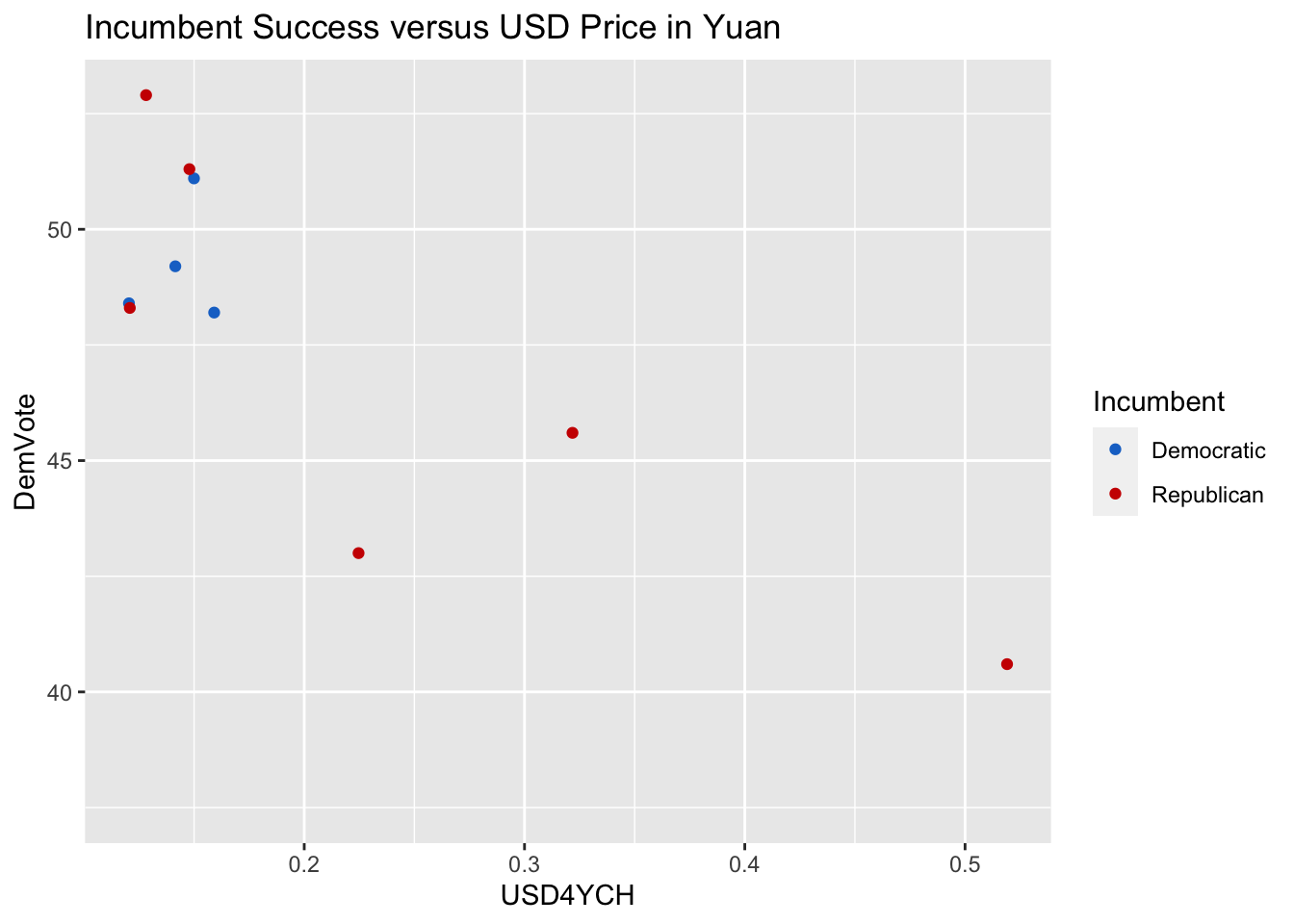
yuan_plot <- ggplot(data=election_outcomes) + geom_point(aes(x=USD4YCH, y=DemVote, color=Incumbent)) + scale_color_manual(breaks = c("Democratic", "Republican"), values = c("dodgerblue3", "red3")) + ggtitle("Incumbent Success versus USD Price in Yuan")
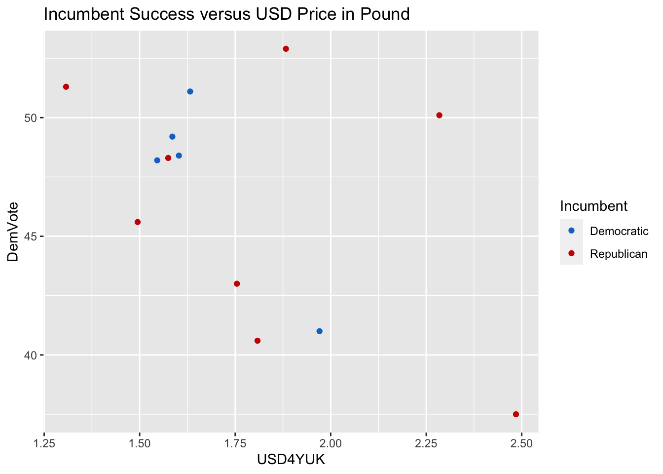
lb_plot <- ggplot(data=election_outcomes) + geom_point(aes(x=USD4YUK, y=DemVote, color=Incumbent)) + scale_color_manual(breaks = c("Democratic", "Republican"), values = c("dodgerblue3", "red3")) + ggtitle("Incumbent Success versus USD Price in Pound")
euro_plot <- ggplot(data=election_outcomes) + geom_point(aes(x=USD4YEU, y=DemVote, color=Incumbent)) + scale_color_manual(breaks = c("Democratic", "Republican"), values = c("dodgerblue3", "red3")) + ggtitle("Incumbent Success versus USD Price in Euro")
yen_plot
yuan_plot
lb_plot
euro_plot
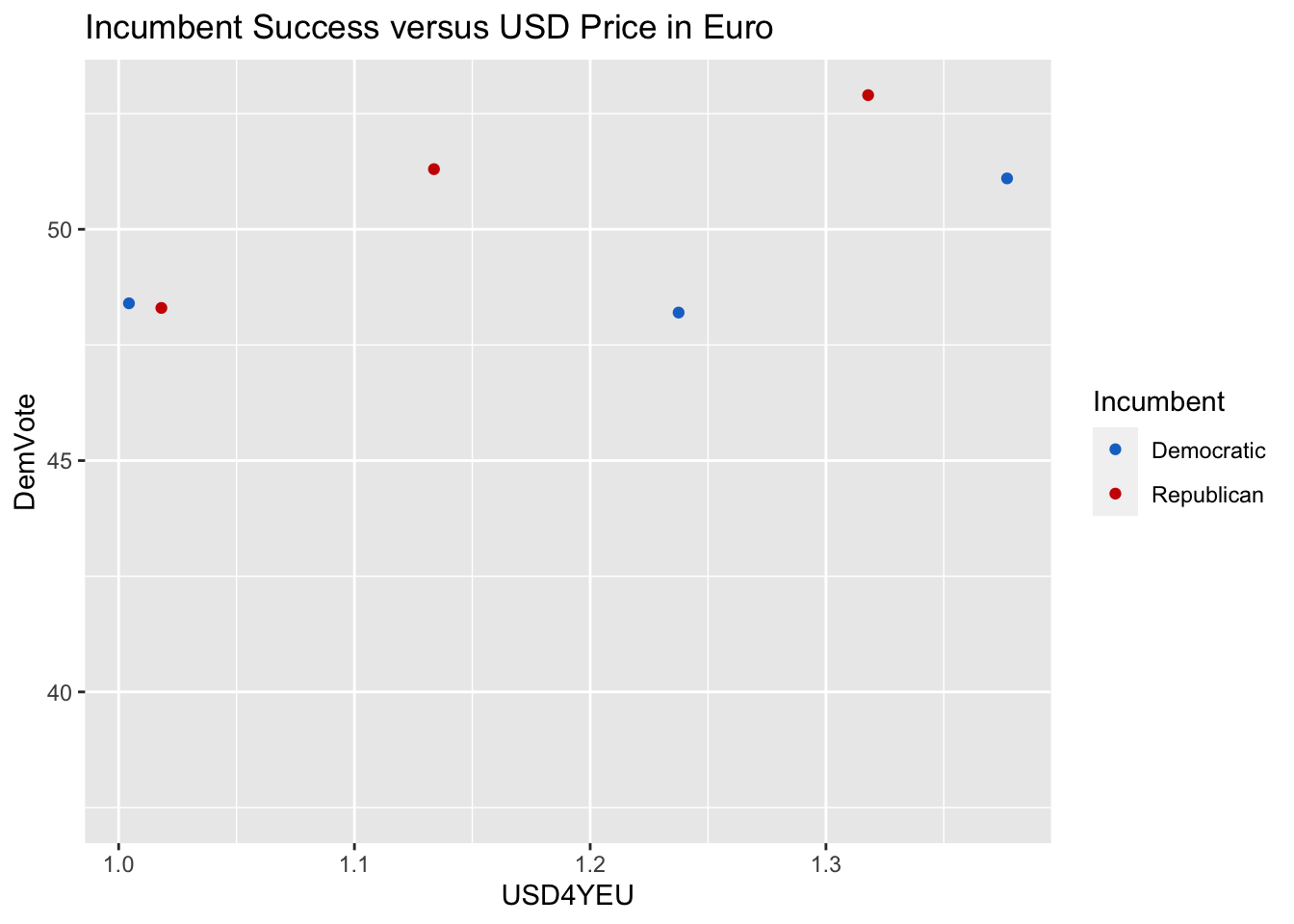
The higher the value on the X-axis, the weaker the U.S. Dollar. The color of the points corresponds to the incumbent candidate. The meanings of the dot colors and vote share values are summarized in the table below:
| Red Dot | Blue Dot | |
|---|---|---|
| Democratic Vote > 50 | Incumbent Unpopular | Incumbent Popular |
| Democratic Vote < 50 | Incumbent Popular | Incumbent Unpopular |
Here are analogous plots for the one-year average values of each currency and how they correspond to incumbent performance/Democratic vote share.
yen_plot1y <- ggplot(data=election_outcomes) + geom_point(aes(x=USD1YJP, y=DemVote, color=Incumbent)) + scale_color_manual(breaks = c("Democratic", "Republican"), values = c("dodgerblue3", "red3")) + ggtitle("Incumbent Success versus USD Price in Yen")
yuan_plot1y <- ggplot(data=election_outcomes) + geom_point(aes(x=USD1YCH, y=DemVote, color=Incumbent)) + scale_color_manual(breaks = c("Democratic", "Republican"), values = c("dodgerblue3", "red3")) + ggtitle("Incumbent Success versus USD Price in Yuan")
lb_plot1y <- ggplot(data=election_outcomes) + geom_point(aes(x=USD1YUK, y=DemVote, color=Incumbent)) + scale_color_manual(breaks = c("Democratic", "Republican"), values = c("dodgerblue3", "red3")) + ggtitle("Incumbent Success versus USD Price in Pound")
euro_plot1y <- ggplot(data=election_outcomes) + geom_point(aes(x=USD1YEU, y=DemVote, color=Incumbent)) + scale_color_manual(breaks = c("Democratic", "Republican"), values = c("dodgerblue3", "red3")) + ggtitle("Incumbent Success versus USD Price in Euro")
yen_plot1y
yuan_plot1y
lb_plot1y
euro_plot1y
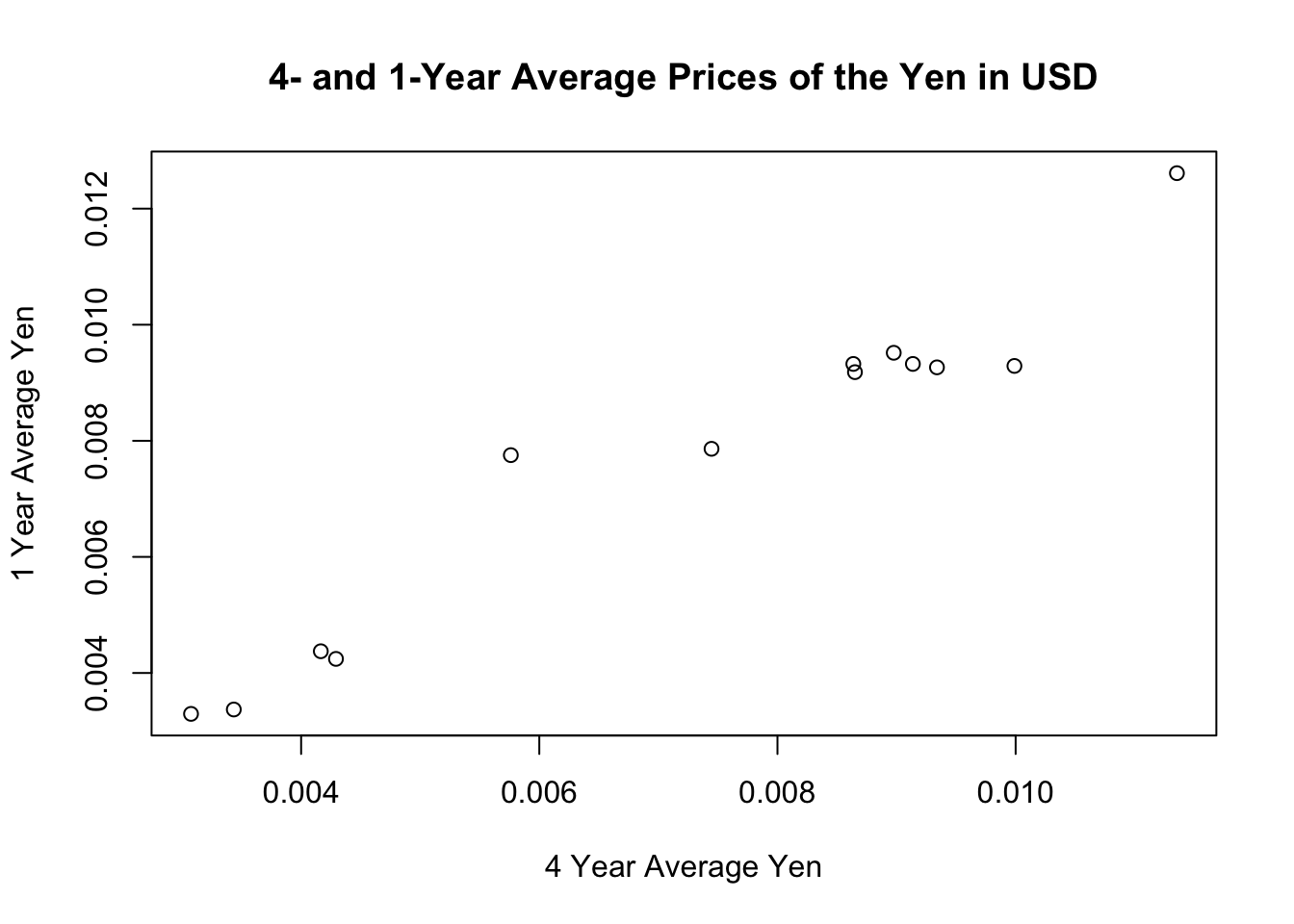
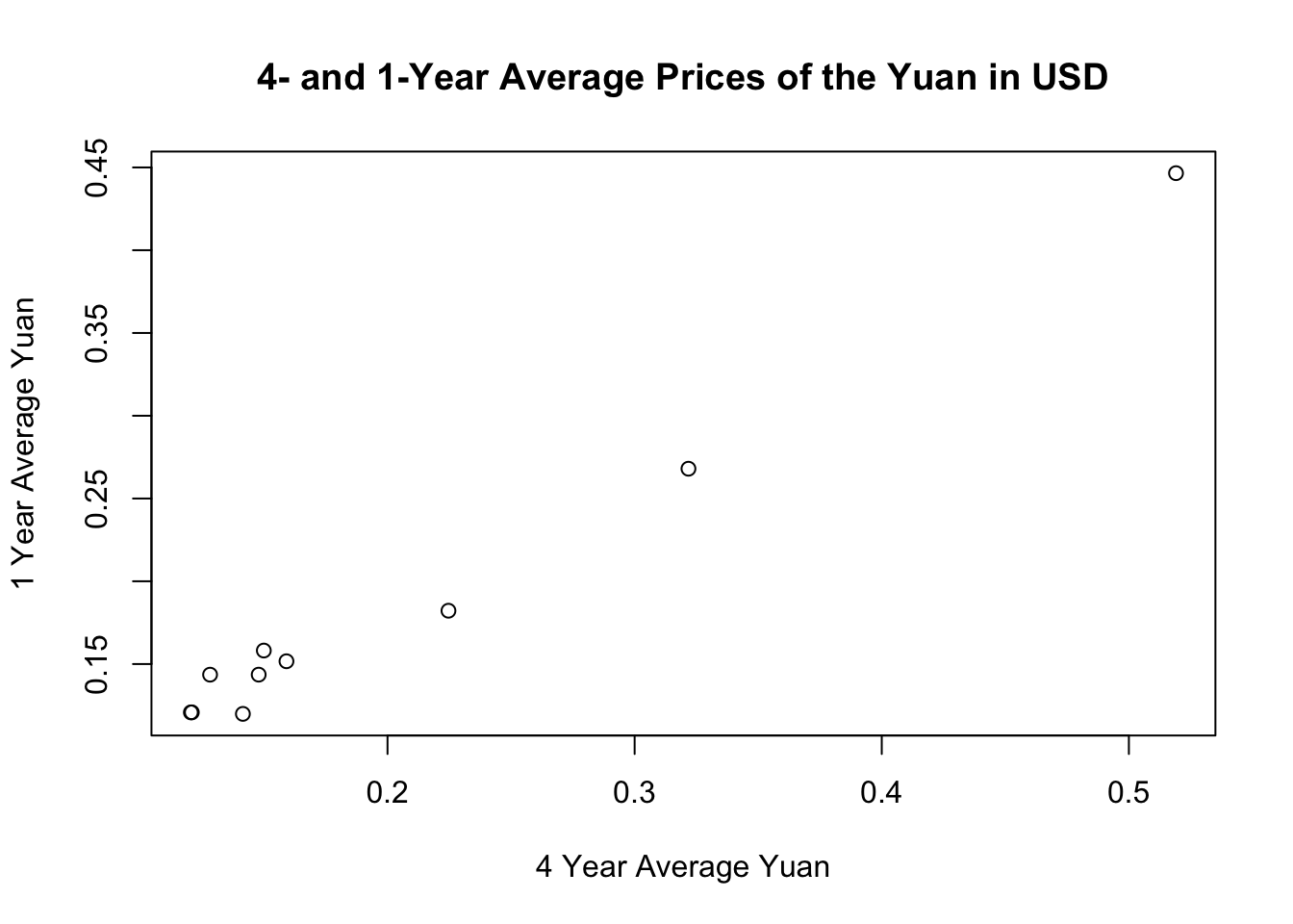
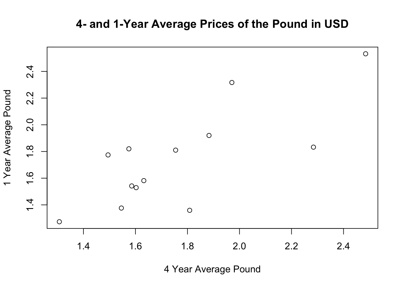
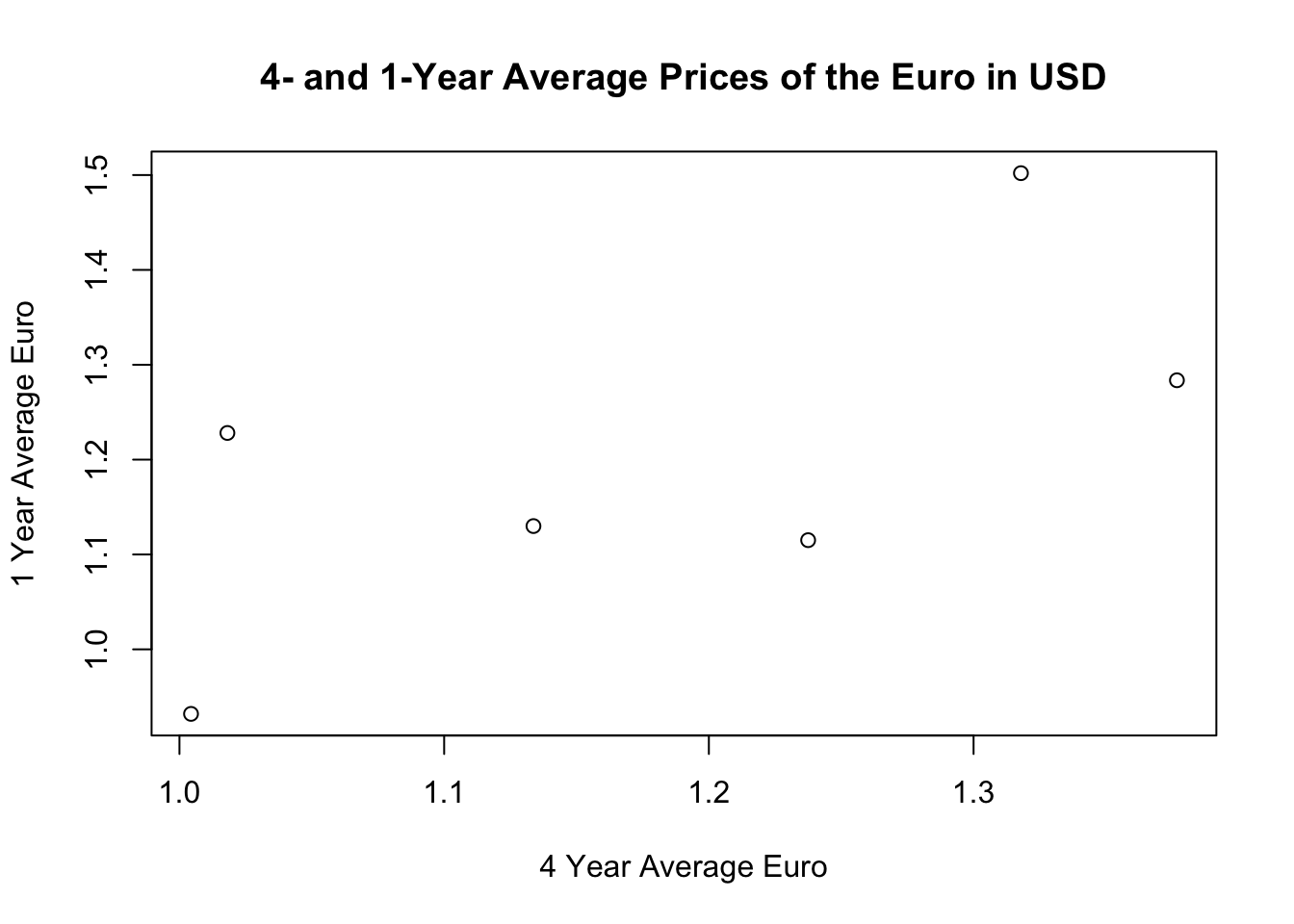
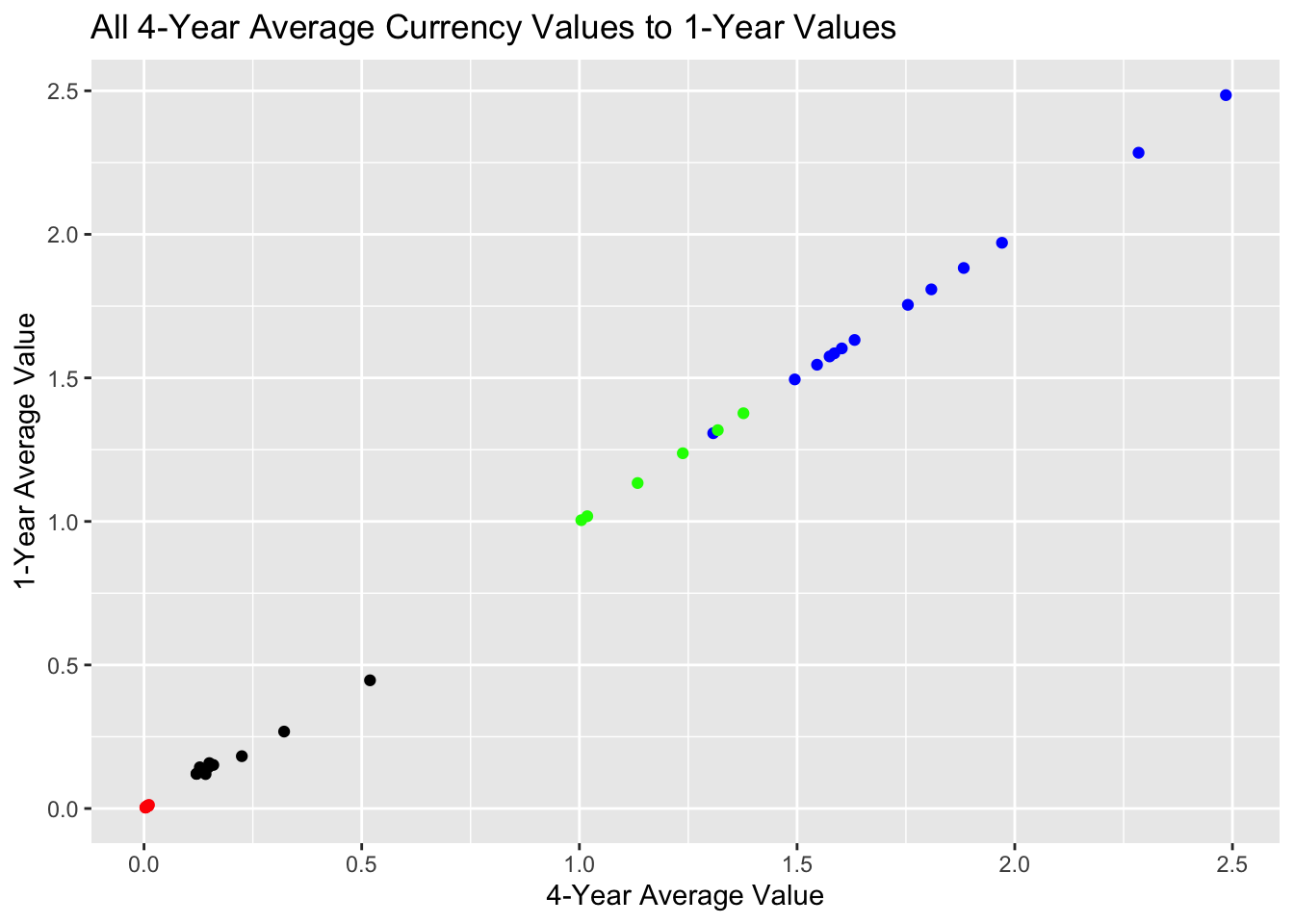
I immediately noticed similarities between the first set of four plots and the second, on a currency-by-currency basis. That is, the plots of election outcomes based on the 4-year average and 1-year average values of the Yen look similar. And likewise for the Yuan, Pound, and Euro respectively. To verify this, I plotted the relationship between the 4-year and 1-year average values of each currency. In each case, I observe a positive correlation.
plot(election_outcomes$USD4YJP, election_outcomes$USD1YJP, xlab="4 Year Average Yen", ylab="1 Year Average Yen", main="4- and 1-Year Average Prices of the Yen in USD")
plot(election_outcomes$USD4YCH, election_outcomes$USD1YCH, xlab="4 Year Average Yuan", ylab="1 Year Average Yuan", main="4- and 1-Year Average Prices of the Yuan in USD")
plot(election_outcomes$USD4YUK, election_outcomes$USD1YUK, xlab="4 Year Average Pound", ylab="1 Year Average Pound", main="4- and 1-Year Average Prices of the Pound in USD")
plot(election_outcomes$USD4YEU, election_outcomes$USD1YEU, xlab="4 Year Average Euro", ylab="1 Year Average Euro", main="4- and 1-Year Average Prices of the Euro in USD")
ggplot(data = election_outcomes) +
  geom_point(mapping=aes(x=USD4YJP, y=USD1YJP), color="red") +
  geom_point(mapping=aes(x=USD4YCH, y=USD1YCH), color="black") +
  geom_point(mapping=aes(x=USD4YUK, y=USD4YUK), color="blue") +
  geom_point(mapping=aes(x=USD4YEU, y=USD4YEU), color="green") +
  xlab("4-Year Average Value") +
  ylab("1-Year Average Value") +
  ggtitle("All 4-Year Average Currency Values to 1-Year Values")
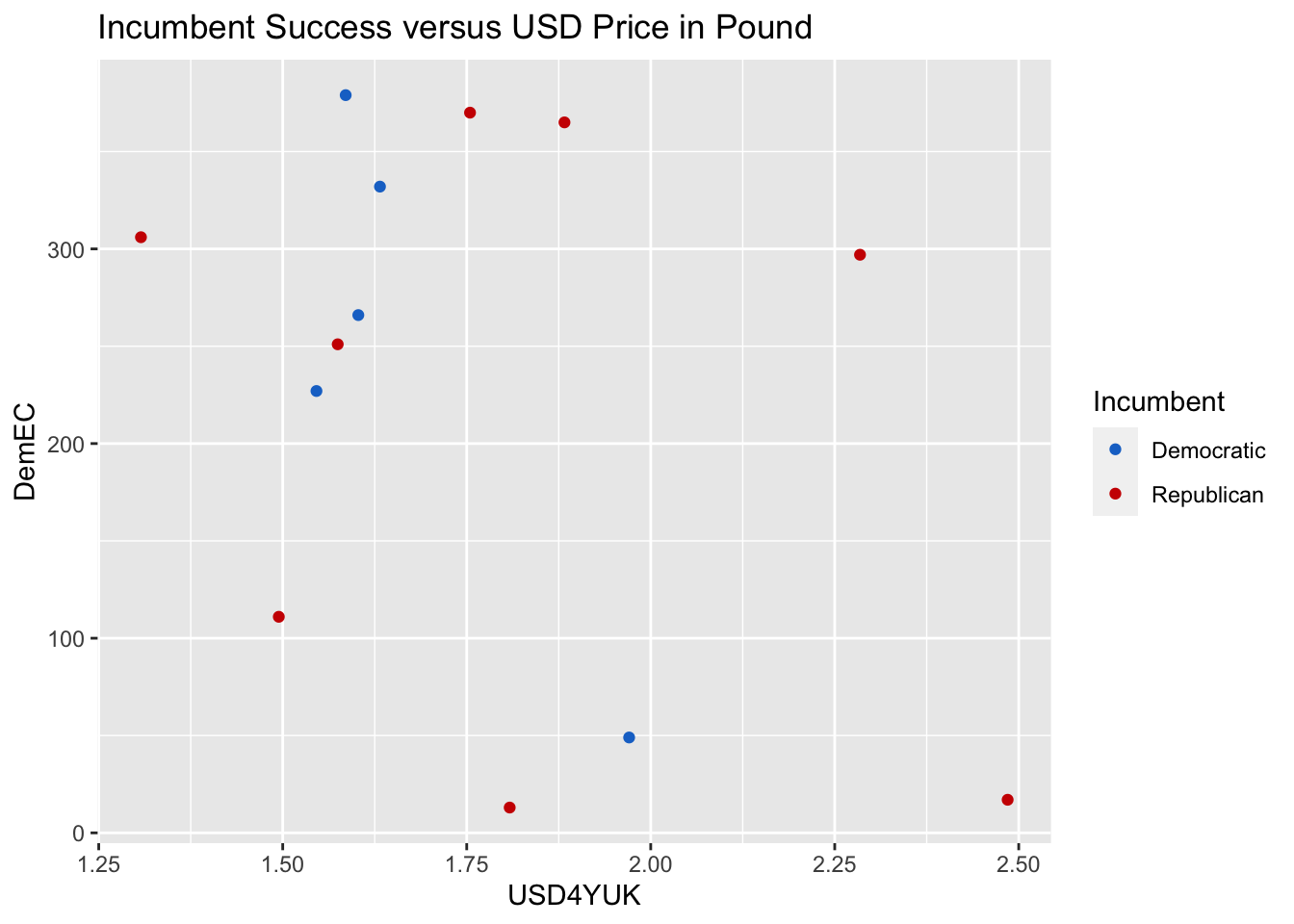
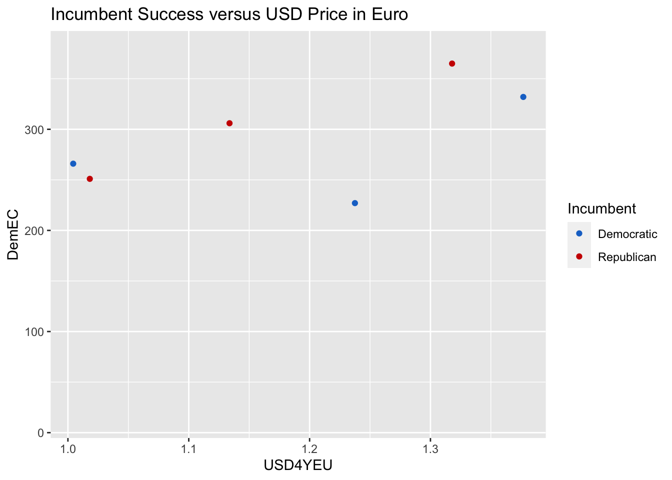
Visually it seems that the Yen and the Yuan are the strongest indicators of Democratic Vote Share. There does not seem to be any correlation between Democratic Vote Share and the value of the USD relative to the Pound or Euro. When the USD is strong relative to the Yen, incumbent Republicans tended to perform well. When it’s weak relative to the Yen, Democrats performed better regardless of the incumbent’s party. It’s worth noting that when there was an incumbent Democratic president, the USD was consistently weak relative to the Yen. When the U.S. Dollar was strong relative to the Yuan, Democrats tended to perform better. Each time there was a Democratic incumbent in this dataset, the Yuan was strong.
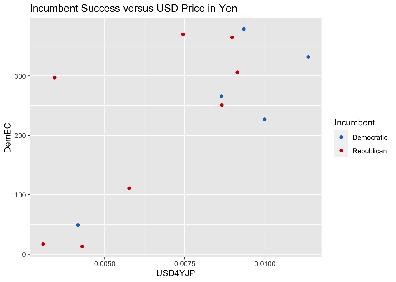
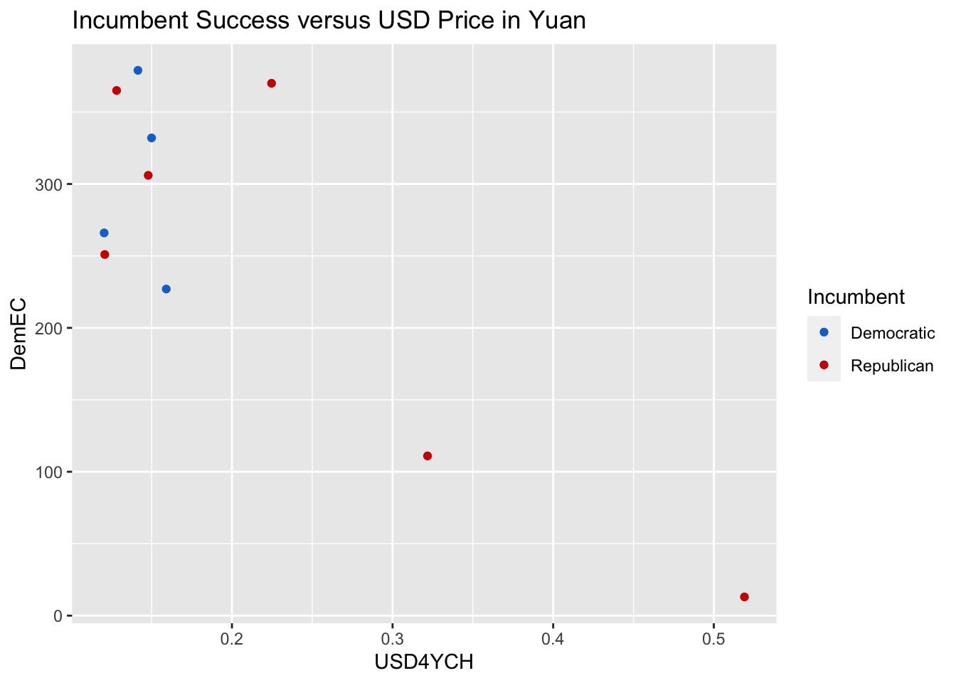
Below, I investigate whether the value of the USD in terms of Yen and Yuan also correlate with the number of electoral votes received. I chose to only plot the 4-year average USD Value versus number of votes received by Democrats in the Electoral College since the trends looked similar to those observed with the popular vote share: the Yen and Yuan were slightly more predictive of a candidate’s success than the Euro and Pound. The main difference is that the values of electoral votes received in each election are more variable than those for Popular Vote Share, which makes sense because Vote Share is measured as a continuous percentage between 1 and 100 and number of Electoral Votes has a discrete number of possible values, theoretically between 0 and 538. Victories in different states can cause major fluctuations to electoral vote share, which also helps explain the increased variance.
# Electoral Plots 1 Year
yen_plot4y_ec <- ggplot(data=election_outcomes) + geom_point(aes(x=USD4YJP, y=DemEC, color=Incumbent)) + scale_color_manual(breaks = c("Democratic", "Republican"), values = c("dodgerblue3", "red3")) + ggtitle("Incumbent Success versus USD Price in Yen")
yuan_plot4y_ec <- ggplot(data=election_outcomes) + geom_point(aes(x=USD4YCH, y=DemEC, color=Incumbent)) + scale_color_manual(breaks = c("Democratic", "Republican"), values = c("dodgerblue3", "red3")) + ggtitle("Incumbent Success versus USD Price in Yuan")
lb_plot4y_ec <- ggplot(data=election_outcomes) + geom_point(aes(x=USD4YUK, y=DemEC, color=Incumbent)) + scale_color_manual(breaks = c("Democratic", "Republican"), values = c("dodgerblue3", "red3")) + ggtitle("Incumbent Success versus USD Price in Pound")
euro_plot4y_ec <- ggplot(data=election_outcomes) + geom_point(aes(x=USD4YEU, y=DemEC, color=Incumbent)) + scale_color_manual(breaks = c("Democratic", "Republican"), values = c("dodgerblue3", "red3")) + ggtitle("Incumbent Success versus USD Price in Euro")
yen_plot4y_ec
yuan_plot4y_ec
lb_plot4y_ec
euro_plot4y_ec
Since the value of the Yen and the Yuan had the most visible association with Democratic Vote Share, I fit two linear models to predict Democratic Vote share based on each of them. I examined the correlation coefficients and \(R^2\) values, and then used the models to predict Democratic Vote Share in 2024.
# lm of Vote Share based on Yen Value
yen_model <- lm(DemVote ~ USD4YJP, data = election_outcomes)
yen_model_1y <- lm(DemVote ~ USD1YJP, data = election_outcomes)
summary(yen_model)
##
## Call:
## lm(formula = DemVote ~ USD4YJP, data = election_outcomes)
##
## Residuals:
##     Min      1Q  Median      3Q     Max
## -4.0438 -1.8952 -0.1390  0.7348  8.1119
##
## Coefficients:
##             Estimate Std. Error t value Pr(>|t|)
## (Intercept)    37.74       2.81  13.429 3.63e-08 ***
## USD4YJP      1236.75     363.95   3.398  0.00595 **
## ---
## Signif. codes:  0 '***' 0.001 '**' 0.01 '*' 0.05 '.' 0.1 ' ' 1
##
## Residual standard error: 3.484 on 11 degrees of freedom
## Multiple R-squared:  0.5121,	Adjusted R-squared:  0.4678
## F-statistic: 11.55 on 1 and 11 DF,  p-value: 0.005949
summary(yen_model_1y)
##
## Call:
## lm(formula = DemVote ~ USD1YJP, data = election_outcomes)
##
## Residuals:
##     Min      1Q  Median      3Q     Max
## -4.1687 -1.9182 -0.4099  0.6183  8.3439
##
## Coefficients:
##             Estimate Std. Error t value Pr(>|t|)
## (Intercept)   37.853      2.871  13.184  4.4e-08 ***
## USD1YJP     1157.912    352.748   3.283   0.0073 **
## ---
## Signif. codes:  0 '***' 0.001 '**' 0.01 '*' 0.05 '.' 0.1 ' ' 1
##
## Residual standard error: 3.545 on 11 degrees of freedom
## Multiple R-squared:  0.4948,	Adjusted R-squared:  0.4489
## F-statistic: 10.78 on 1 and 11 DF,  p-value: 0.007301
Though the 4-year average value of the Yen and 1-year average value of the Yen have collinearity, the result above shows that the 4-year average value of the Yen is a stronger predictor of Democratic Vote Share. Going forward I’ll use the 4-year averages in my models.
# lm of Vote Share based on Yuan
yuan_model <- lm(DemVote ~ USD4YCH, data = election_outcomes)
summary(yuan_model)
##
## Call:
## lm(formula = DemVote ~ USD4YCH, data = election_outcomes)
##
## Residuals:
##     Min      1Q  Median      3Q     Max
## -4.3335 -1.3181  0.1739  1.6075  3.1850
##
## Coefficients:
##             Estimate Std. Error t value Pr(>|t|)
## (Intercept)   52.880      1.439  36.750  3.3e-10 ***
## USD4YCH      -24.688      6.088  -4.055  0.00366 **
## ---
## Signif. codes:  0 '***' 0.001 '**' 0.01 '*' 0.05 '.' 0.1 ' ' 1
##
## Residual standard error: 2.32 on 8 degrees of freedom
##   (3 observations deleted due to missingness)
## Multiple R-squared:  0.6727,	Adjusted R-squared:  0.6318
## F-statistic: 16.45 on 1 and 8 DF,  p-value: 0.003657
The Yen’s positive correlation coefficient means that Democrats receive a higher popular vote share when the Yen is strong relative to the USD (i.e. 1 Yen is more expensive in terms of USD). The Yuan’s negative coefficient means that when the Dollar is strong relative to the Yuan, Democratic candidates receive a higher popular vote share. The Yuan Model has a higher value for \(R^2\) meaning that changes in the value of the Yuan are better at explaining changes in the popular vote share than changes in the Yen.
Out of curiosity, I decided to fit two models, again based on the 4-year average values of the Yen and Yuan, to predict electoral college outcomes in 2024. The Yuan’s higher value for \(R^2\) again indicates that it has stronger predictive power than the Yen.
# fit 2 models to predict electoral college outcomes
yen_model_ec <- lm(DemEC ~ USD4YJP, data=election_outcomes)
yuan_model_ec <- lm(DemEC ~ USD4YCH, data=election_outcomes)
summary(yen_model_ec)
##
## Call:
## lm(formula = DemEC ~ USD4YJP, data = election_outcomes)
##
## Residuals:
##     Min      1Q  Median      3Q     Max
## -112.66  -66.18  -27.59   74.98  201.45
##
## Coefficients:
##             Estimate Std. Error t value Pr(>|t|)
## (Intercept)   -24.97      80.28  -0.311   0.7616
## USD4YJP     35090.36   10396.85   3.375   0.0062 **
## ---
## Signif. codes:  0 '***' 0.001 '**' 0.01 '*' 0.05 '.' 0.1 ' ' 1
##
## Residual standard error: 99.53 on 11 degrees of freedom
## Multiple R-squared:  0.5087,	Adjusted R-squared:  0.4641
## F-statistic: 11.39 on 1 and 11 DF,  p-value: 0.006196
summary(yuan_model_ec)
##
## Call:
## lm(formula = DemEC ~ USD4YCH, data = election_outcomes)
##
## Residuals:
##     Min      1Q  Median      3Q     Max
## -75.347 -60.147  -1.025  40.401 124.629
##
## Coefficients:
##             Estimate Std. Error t value Pr(>|t|)
## (Intercept)   420.55      44.22   9.510 1.23e-05 ***
## USD4YCH      -779.76     187.11  -4.167  0.00313 **
## ---
## Signif. codes:  0 '***' 0.001 '**' 0.01 '*' 0.05 '.' 0.1 ' ' 1
##
## Residual standard error: 71.3 on 8 degrees of freedom
##   (3 observations deleted due to missingness)
## Multiple R-squared:  0.6846,	Adjusted R-squared:  0.6452
## F-statistic: 17.37 on 1 and 8 DF,  p-value: 0.003133
# prediction
data_2024 <- subset(all_currencies, YEAR %in% c(2021, 2022, 2023, 2024))
avg_JP <- mean(data_2024$DEXUSJP, na.rm=TRUE)
avg_CH <- mean(data_2024$DEXUSCH, na.rm=TRUE)

yen_pred <- predict(yen_model, newdata=data.frame(USD4YJP=avg_JP))
yuan_pred <- predict(yuan_model, newdata=data.frame(USD4YCH=avg_CH))
cat("Projected Democratic Vote Share Based on USD Value Relative to the JPN Yen: ", yen_pred)
## Projected Democratic Vote Share Based on USD Value Relative to the JPN Yen: 47.27305
cat("Projected Democratic Vote Share Based on USD Value Relative to the CHN Yuan: ", yuan_pred)
## Projected Democratic Vote Share Based on USD Value Relative to the CHN Yuan: 49.26073
yen_pred_ec <- predict(yen_model_ec, newdata=data.frame(USD4YJP=avg_JP))
yuan_pred_ec <- predict(yuan_model_ec, newdata=data.frame(USD4YCH=avg_CH))
cat("Projected Democratic Electoral College Votes Based on USD Value Relative to the JPN Yen: ", yen_pred_ec)
## Projected Democratic Electoral College Votes Based on USD Value Relative to the JPN Yen: 245.5026
cat("Projected Democratic Electoral College Votes Based on USD Value Relative to the CHN Yuan: ", yuan_pred_ec)
## Projected Democratic Electoral College Votes Based on USD Value Relative to the CHN Yuan: 306.2406
Interestingly, the shares of the electoral college predicted by the the value of the USD relative to the Yen and the Yuan were vastly different from each other–so different that, in a model based on the Yen, the Republican Candidate (Trump) would win the electoral college and in a model based on the Yuan, the Democratic Candidate (Harris) would win the electoral college. In terms of the popular vote share, both the models based on the Yen and the Yuan showed the Democratic candidate receiving under 50%.
Extension Section: Heterogenous Predictive Power of the Economy
This section zooms in on the difference in the effect of the value of the U.S. Dollar for predicting incumbent victories versus challenger victories. I separate the data into elections won by incumbents and elections won by challengers. Then, I fit linear models using the Yen and the Yuan, respectively, to see if they were better at predicting incumbent shares of the popular vote or challenger shares of the popular vote. I chose to predict shares of the popular vote because the set of values it can take on is smaller and I'm working with smaller sample sizes in this section. Given that there have only been 13 U.S. presidential elections since 1971, the sample size was already small. Once I split the data between incumbent victories and challenger wins, I deal with two even smaller subsets, which is a limitation.# split the data
election_outcomes <- election_outcomes %>%
mutate(winner = case_when(DemEC >= 270 ~ "Democratic",
RepEC >= 270 ~ "Republican"))
# incumbent successes, challenger successes
incumbent_wins <- subset(election_outcomes, Incumbent == winner)
challenger_wins <- subset(election_outcomes, Incumbent != winner)
# fit linear models
inc_yen_model <- lm(DemVote ~ USD4YJP, data=incumbent_wins)
inc_yuan_model <- lm(DemVote ~ USD4YCH, data=incumbent_wins)
chal_yen_model <- lm(DemVote ~ USD4YJP, data=challenger_wins)
chal_yuan_model <- lm(DemVote ~ USD4YCH, data=challenger_wins)
# compare correlation coefficients and R^2
ext_results <- data.frame(c("Incumbent Performance Based on Yen", "Incumbent Performance Based on Yuan", "Challenger Performance Based on Yen", "Challenger Performance Based on Yuan"), c(inc_yen_model$coefficients["USD4YJP"], inc_yuan_model$coefficients["USD4YCH"], chal_yen_model$coefficients["USD4YJP"], chal_yuan_model$coefficients["USD4YCH"]), c(summary(inc_yen_model)$r.squared, summary(inc_yuan_model)$r.squared, summary(chal_yen_model)$r.squared, summary(chal_yuan_model)$r.squared))
colnames(ext_results) <- c("Model", "Coefficients", "R-Squared")
ext_results
##                                  Model Coefficients R-Squared
## 1   Incumbent Performance Based on Yen   1600.69279 0.9349441
## 2  Incumbent Performance Based on Yuan    -22.74748 0.9062180
## 3  Challenger Performance Based on Yen    715.04056 0.1801265
## 4 Challenger Performance Based on Yuan    -76.17687 0.6925921
As is evident in the table above, The Yen is much more predictive of incumbent candidate vote share than of challenger vote share. The Yuan is likewise more predictive of incumbent vote share. This is interesting, and somewhat intuitive because because it addresses the phenomenon that many candidates spend their first term in office focused on domestic policy and their second term on foreign policy. If this is well-known in the electorate, it may make voters more cognizant of international exchange rates when voting for an incumbent than when voting for a first-term president.